A couple of weeks ago we saw the blog post visualizing the voting patterns in the Polish parliament. In anticipation of the upcoming election and in the interest of checking up on our elected representatives we thought we would do a similar analysis for the Norwegian parliament. First we will visualize a projection of the voting data of the Norwegian parliament into 3D, and then we will try to interpret the axes of the projection in terms of the issues voted on.

The data

Stortinget, the Norwegian parliament, has a nice web service for retrieving details about the process an issue passes through in the parliament. Proposals, committees, referendums and so on; there is a surprising amount of detail in there. With a bit of work we pulled out the individual votes for the parliamentary referendums we were able to access. On the less bright side the data doesn’t appear to be complete as far as we can see, and there is also a range of documented caveats and restrictions regarding which votes are actually registered in the system. This reduces the usefulness of any detailed analysis based on this data, but we still think the aggregated picture one can create is both interesting and valid.

The voting data comes in the form of for, against or abstained votes. Like in the referenced blog post we would like to visualize the similarity in voting patterns for the representatives. In order to do this we constructed a grid of referendums versus representatives for the current parliamentary period with a single cell representing a vote encoded as 1 for “for”, -1 for “against” and 0 if “abstained” which makes this a neutral midpoint in the analysis we are going to do. This gives a data point for each representative in the multidimensional “vote space” where we can do things like clustering or similarity measures to find patterns in the votes.

Visualizing the vote space

Since we have the records for 58 referendums so far in the 2013-2017 period and 612 records in the 2009-2013 period we cannot directly visualize our representatives in the vote space. There are several techniques for projecting data like this into lower dimensional sub-spaces while still retaining the essential characteristics of the data. In this blog post we will project the voting data into 3 dimensions using Principal Components Analysis. There are several alternatives here and we chose PCA for the following reasons.

• Our data is categorical, but non-binary. It is also distributed symmetrically with 0 representing a neutral value. One would expect that categorical data would not necessarily be modeled well by PCA, but the symmetry and the consistent values involved combined with the density of the data suggests that PCA should behave well.
• PCA is based on Singular Value Decomposition (SVD) of the co-variance matrix and consequently has properties that are straightforward to interpret compared to methods such as Multidimensional Scaling (MDS) which seeks to preserve the individual distances between data points.
• PCA gives us a projection along axes which have the most variance which in our case should highlight the parts of the data where there is less agreement between parties or representatives. This disagreement is the sort of contrast that we seek to visualize.
• PCA axes are linear combinations of the separate referendums which means we can create a comprehensible interpretation of the visualization in terms of political issues.

Other methods are generally harder to interpret with regard to their applicability and the resulting projections (like probabilistic methods such as ICA) or don’t highlight the contrast we want to visualize (like MDS which preserves the distance relationships between the representatives).

The plots

We’re just going to present the plots without any political commentary. The first plot is for the current parliamentary period while the second is for the previous period. In the first we have highlighted Miljøpartiet De Grønne which only has a single representative in the current parliament. It is interesting to note the coherence of certain coalition partners in government and the location of the centrist parties. An important measure for the PCA projection is the explained variance ratio of the axes. This is the amount of variance that is preserved in the projected axes and is a measure of how much of the original information is retained in the projection. For our plots the total explained variance is ca. 62% and 57% which means there is quite a bit of diversity in the voting patterns that is not shown in the plot but still enough to consider them informative. The axes are ordered by explained variance so that the first axis explains over 40% of the variance while the remaining two around 10% each.

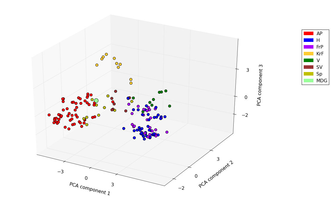
Projection of voting patterns in the 2013-2015 parliamentary periods.

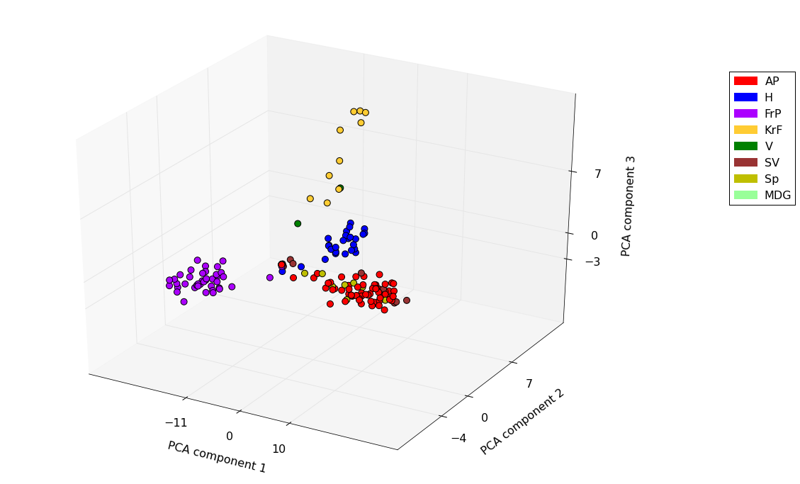
Projection of voting patterns in the 2009-2013 parliamentary periods.

Interpreting the projection axes

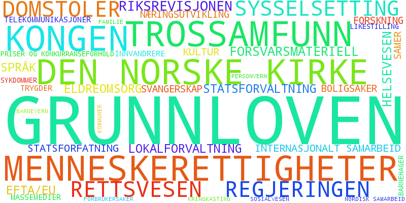
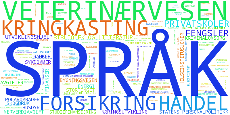
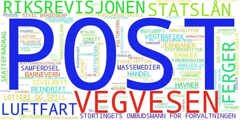
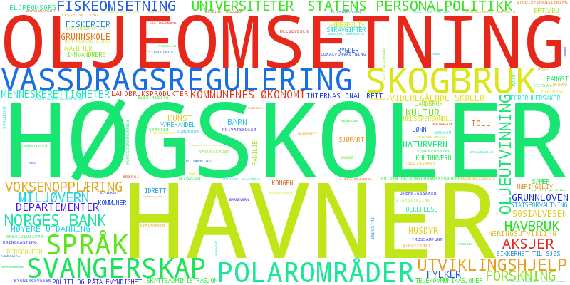
In and of itself the colorful dots have a limited story to tell. If we could characterize what the axes in the graphs represent we could draw more interesting and detailed inferences. What we will do here is mostly for illustrative purposes though, since it really requires someone knowledgeable in Norwegian parliamentary politics and procedure to build an analysis with proper grounding in actual political activity. Here we will just play around with the data. It is tempting to treat the positive and negative directions of the axes as affirmative/negative on an issue but we would have to look at the text for each referendum to see what “for” and “against” actually means with regards to the sentiment on each issue. Actually the same issue tend to have both strong positive and negative components in a projected axis which strongly suggests that there isn’t a single sentiment expressed by the axis direction. Can we create a credible summary of the axes without closely studying each referendum and each issue? Each referendum is part of an issue and it turns out each issue has a list of topics associated with it. So we can make a summary of how much each topic is represented in an axis by the weight for each vote on this issue in a given axis. Each axis is a linear component of the votes and we add up the absolute value of each vote that is part of an issue concerning the topic. To class up this blog a bit we decided to make a word cloud out of the results.

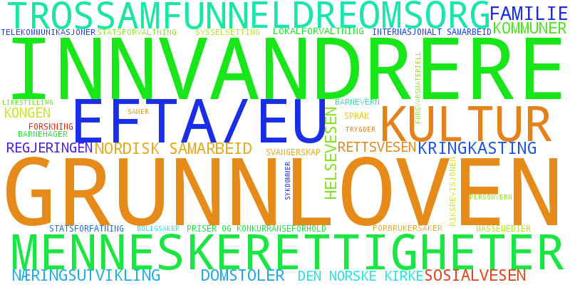
Word cloud for PCA component 1 for the 2013-2015 plot.

Word cloud for PCA component 2 for the 2013-2015 plot.

Word cloud for PCA component 3 for the 2013-2015 plot.

The most characteristic topics

Some topics account for most of the activity in parliament and tend to dominate the data if we look only at the volume of votes. For the present parliamentary period the data is rather sparse so this isn’t as pronounced in the word clouds, but for the 2009-2013 period where there is a lot more data transportation/communication and health dominates in all the axes. Can we see what topics are characteristic for an axis instead? To highlight topics that have a high overall weight in our projection in comparison to their overall presence in the referendums we weigh each topic by its “Inverse Topic Frequency” – similar to the common Inverse Document Frequency (IDF) common in search relevance and information retrieval. This makes rarer but highly weighted topics stand out. This weighting gives us a clearer picture of how the axes differ from each other, even if they don’t necessarily show the ratio of influence of these topics on the projection itself.

Contrastive word cloud for PCA component 1 for the 2009-2013 plot.

Contrastive word cloud for PCA component 2 for the 2009-2013 plot.

Contrastive word cloud for PCA component 3 for the 2009-2013 plot.

Wrapping up

While the plots shown here are both interesting and entertaining there are many possibilities available when creating these visualizations and interpreting them. Consequently while they can be very helpful during analysis and point out interesting directions one might not have noticed otherwise, a purely quantitative analysis can fall prey to  “researchers degrees of freedom” and steer conclusions towards predetermined biases and worse. External validation and domain expertise can help ground models and inferences in reality. With the help of a domain expert we could shape the data into a format more amenable for analysis, for example by weighting issues by importance and normalizing the vote sentiment across referendums. This would provide us with a much firmer foundation for making inferences than the raw data by itself as we have done here.