How Elasticsearch calculates significant terms
The magic of the “uncommonly common”.
Many of you who use Elasticsearch may have used the significant terms aggregation and been intrigued by this example of fast and simple word analysis. The details and mechanism behind this aggregation tends to be kept rather vague however and couched in terms like “magic” and the commonly uncommon. This is unfortunate since developing informative analyses based on this aggregation requires some adaptation to the underlying documents especially in the face of less structured text. Significant terms seems especially susceptible to garbage in – garbage out effects and developing a robust analysis requires some understanding of the underlying data. In this blog post we will take a look at the default relevance score used by the significance terms aggregation, the mysteriously named JLH score, as it is implemented in Elasticsearch 1.5. This score is especially developed for this aggregation and experience shows that it tends to be the most effective one available in Elasticsearch at this point.
The JLH relevance scoring function is not given in the documentation. A quick dive into the code however and we find the following scoring function.
\frac{p_{fore}}{p_{back}} & p_{fore} - p_{back} > 0 \\ 0 & elsewhere \end{matrix}\right.")
Here the 

Expanding the formula gives us the following which is quadratic in
\frac{p_{fore}}{p_{back}} = \frac{p_{fore}^2}{p_{back}} - p_{fore}")
By keeping
On the face of it this looks bad for a scoring function. It can be undesirable that it changes sign, but more troublesome is the fact that this function is not monotonically increasing.
The gradient of the function:
 = \left(\frac{2 p_{fore}}{p_{back} - 1} , -\frac{p_{fore}^2}{p_{back}^2}\right)")
Setting the gradient to zero we see by looking at the second coordinate that the JLH does not have a minimum, but approaches it when

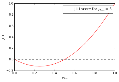
Furtunately the decreasing part of the function is in an area where 

With this it seems sensible to just drop the linear term of the JLH score and just use the quadratic part. This will result in the same ranking with a slightly less steep increase in score as

Looking at the level sets for the JLH score there is a quadratic relationship between the 

Where the negative part is outside of function definition area.
This is far easier to see in the simplified formula.

An increase in

As we see the score increases sharply as
Finally a 3D plot of the score function.
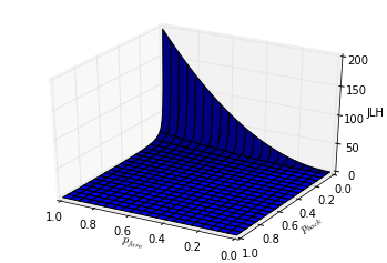
So what can we take away from all this? I think the main practical consideration is the squared relationship between
The results and visualizations in this blog post is also available as an iPython notebook.


Nice write up. I plotted some of the other scoring heuristics here: https://twitter.com/elasticmark/status/513320986956292096
For me, the choice of scoring function is essentially a question of emphasis between precision and recall. If I analyse the results of a search for “Bill Gates” do I suggest “Microsoft” or “bgC3″ as the most significant terms? The rarer bgc3 is more closely allied (so high precision) but perhaps of less practical use due to poor recall. The inverse is true of Microsoft.
Putting aside the question of precision/recall emphasis, I found the following features do the most to improve significance suggestions on text:
1) Removal of duplicate/near duplicate text in the results being analysed
2) Discovery of phrases
3) Analysing top-matching samples not all content (see the new “sampler” agg)
4) “Chunking” documents e.g. into sentence-docs if the foreground sample of docs is low in number.
Additionally, text analysis in elasticsearch should ideally not be reliant on field data to avoid memory issues.
These approaches are a little detailed to get into here but are important parts of improving elasticsearch’s significance algos on free text.
The mystery of “JLH” is my daughter’s initials :)
Cheers,
Mark
Ayup, thanks letting us in on the name and mentioning the new sampler aggregation :) That looks quite interesting.
The precision/recall viewpoint is indeed illuminating. I tend to shy away from it since it feels tied to specific task or goal. I’m not really sure I would call bgC3 more precise than Microsoft in this case, although bgC3 probably points to a more limited set of documents. It’s all in the context I guess.
If you can structure your data in a manner that supports your task that is certainly a good idea. Chunking up words I feel is something that has to be done with more care. Pure collocational or n-gram approaches can end up emphasizing turns of phrase without interesting content, you might call them phrase stopwords. I’ld be more inclined to extract meaningful multiword units such as verb complexes or entities.
Doing sentence/paragraph docs incurs indexing costs and seem to me to be a poor mans estimate of the term-frequency. It’s certainly a practical solution but it would nice if there was an option for using the TF in the significant terms aggregation for foreground sets where it is feasible.
Anyhow, thanks for putting cool stuff like this into Elasticsearch and hope you’ll find ways to make significant terms into an even more precise and flexible tool than it is today.
Snakkes!
André